Discovering Bayesian Optimization

How I got into Bayesian Optimization

While taking the Advanced Machine Learning course at the University of Maryland I got more involved in Bayesian statistics and how they can be applied to data science (Against the Frequentist approach). I could make a long post about the Bayesian vs the Frequentist paradigm but I guess I’ll cover this topic eventually.

One of the things I learned in the field of Bayesian statistics, is Bayesian Optimization. It’s a technique to find optimal values across a complex search space, when navigating this search space (I mean, running an experiment and obtaining a result until we got the optimal value) is very expensive.

I was very surprised by reading how this technique was applied at Meta just to find an optimal concrete formulation. There is no mathematical formula for concrete efficiency, the only way of discovering the best combination is just trying, but each try requires more than 20 days of wait. For a better description of this case you just can see:

Engineering At Meta: Using AI to make lower-carbon, faster-curing concrete

Non-parametric Optimization Methods

Before getting into Bayesian Optimization, I was already familiar with the classic Global Search Methods. Whenever your problem couldn’t be parametrized, or the function wasn’t differentiable, you could use these techniques, among others:

• Genetic Algorithms
• Simulated Annealing
• Particle Swarm Optimization

These techniques are great if testing your problem only takes a few milliseconds, otherwise you’ll lose a lot of time going through the search space blindly.

Bayesian Optimization builds a model of the function to decide where to sample next, and minimize the number of experiments.

Using Bayesian Statistics

Bayesian statistics start with a prior assumption, a set of probabilities. Every time you run an experiment, those probabilities get adjusted, your assumptions start getting better.

This is what we do with Bayesian Optimization. There may not be a mathematical formula to get the most efficient concrete formulation, but there are some rules in the nature, and we’re gonna discover them just through experimentation.

How does Bayesian Optimization Work?

Suppose we want to optimize a black-box function $f(x)$, but we can’t observe it directly, we need to run experiments. We need to consider real-life experiments also have noise. We can model this with a Surrogate Model: $y = f(x) + \epsilon$.

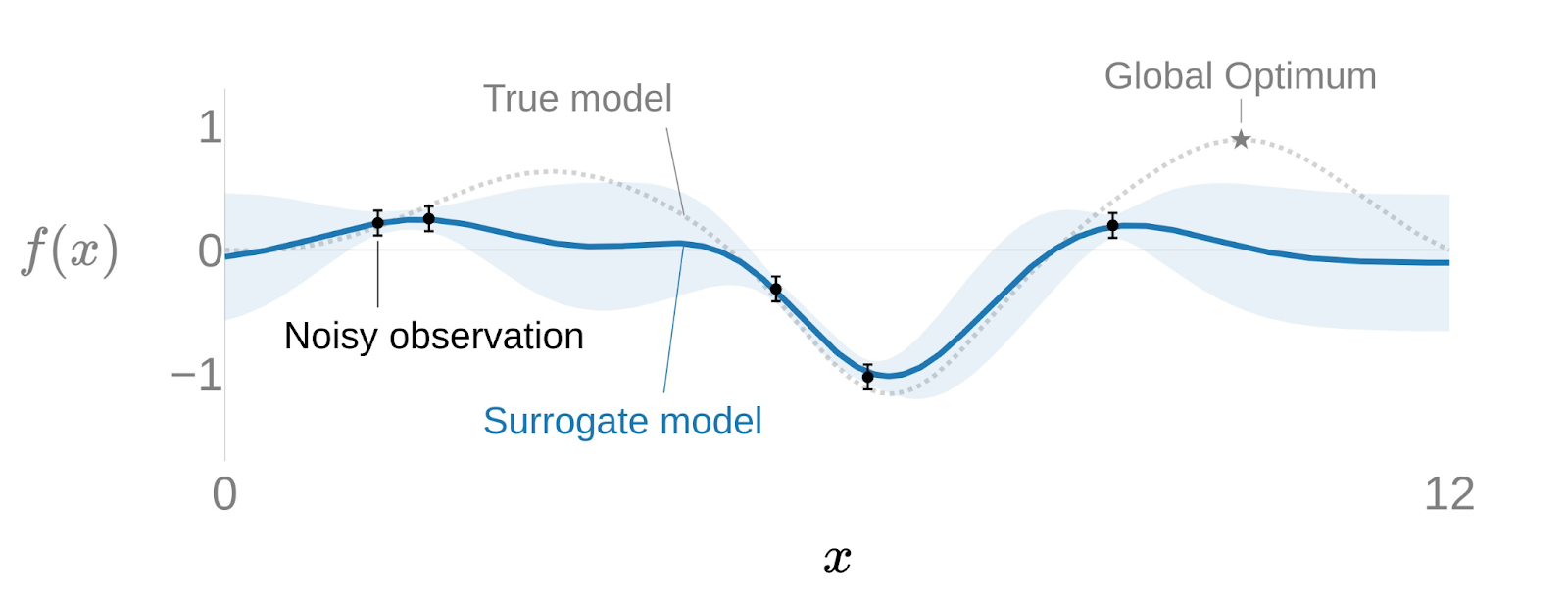
But $f(x)$ is not just a function, it’s a probability model. We don’t know the certain values of this function, we know the probability of them. Remember we’re modelling the real world and the real world is chaotic, not precise.

The best way to represent this kind of “probability function” is with a Gaussian Process, defined as $f(x) \sim GP(m(x), k(x, x'))$, where:

• $m(x)$ is the mean function, the best estimation for the result at that point $x$
• $k(x, x')$ is the covariance function, describes how the different points correlate, basically, the form of this function

The most common covariance function is the Gaussian kernel, for now, we’ll work with this kernel:

$k(x, x') = \sigma^2 \exp\left(-\frac{\|x - x'\|^2}{2l^2}\right)$

How the process works:

• At the beginning of our optimization we know nothing, our Gaussian process will have a high uncertainty.
• We run the experiment with one point $x$, and we obtain $f(x)$. So we adjust the Gaussian Process.
• We keep running experiments and, over time, our function will get more precise.

The Acquisition Function

We have a surrogate model, but we still need to decide which point to test next. Running experiments blindly defeats the purpose - The whole point is to find the optimum with as few tries as possible. The Acquisition Function is what makes that decision: given the current state of the Gaussian Process, it tells us where to sample next to gain the most information.

The surrogate model doesn’t just predict a value at each point - it also estimates how uncertain that prediction is. That uncertainty is the key. We need to get more information about those points on which the uncertainty is higher.

The most widely used acquisition function is the Expected Improvement (EI):

$f^*$ is the best result observed so far, the known optimal value. If other points are expected to give us a higher value we need to evaluate them. That depends on both the expected value of this point and its uncertainty. This function will choose points with high predicted value, high uncertainty, or both.

The following animation provides a good insight of how the surrogate model would get adjusted over each iteration. Notice how after just a few iterations the algorithm has effectively narrowed the search. The algorithm quickly focuses on the most promising areas rather than exhaustively trying on the entire domain.

When to Use It

Bayesian Optimization fits best when two conditions align: the function has no parametric formula, and each evaluation is expensive.

Concrete use cases:

• Hyperparameter tuning: Finding the optimal configuration for a neural network is costly and each training run can take hours. Bayesian Optimization reduces the number of runs needed compared to grid search or random search.
• Adaptive A/B testing: Human behavior is noisy and hard to model analytically. Bayesian models let us identify the best-performing variant with fewer rounds of testing.
• Physical and chemical optimization: Any domain where experiments take days or weeks (Drug formulations, material science, concrete mixing) is a natural fit. The Meta concrete case is one of the clearest examples of this.

Adaptive Experimentation with Ax

The theory above is the foundation. In practice, Meta’s Adaptive Experimentation (Ax) library implements all of this in a clean Python API. It’s the same platform Meta used for the concrete optimization project.

In a follow-up post I’ll walk through a hands-on example using Ax: defining the search space, running the optimization loop, and reading the results.