Frequentist vs Bayesian Statistics

In my previous post on Bayesian Optimization, I mentioned the Bayesian vs. Frequentist paradigm as the foundation behind the technique, and that I would cover it eventually. This is that post.

What’s the Frequentist Approach

If you ever learned about data science, you have surely taken a frequentist approach. Suppose we have a linear regression, the most basic formula in data science:

Where $x$ is the amount of money spent in ads, $y$ is the number of sales, $\beta_0$ and $\beta_1$ are the fixed (but unknown) coefficients we estimate from data, and $\varepsilon$ is the noise term.

In this case, using a simple approach like least squares, we can find the values of $\beta_0$ and $\beta_1$ that best fit a series of given data points.

In a perfect scenario, our data points will look like this:

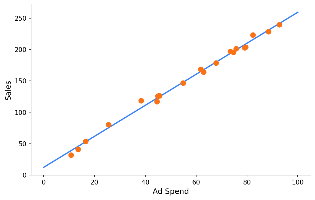
In this case, the intercept $\beta_0$ is 10, and the slope $\beta_1$ is 2.5.

Now, suppose our dataset has more noise:

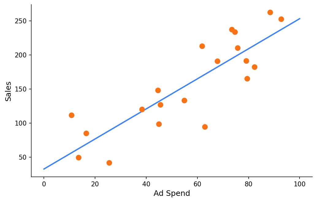
In both cases, the point estimates for intercept and slope produced by a frequentist approach are nearly identical - even though the data clearly contains very different levels of noise. Frequentist statistics do offer confidence intervals and p-values, and a wider CI does reflect less certainty. But a 95% CI doesn’t mean “there is a 95% probability that $\beta_1$ is in this range.” It means: if we repeated this experiment many times, 95% of such intervals would contain the true value. The parameter itself has no probability distribution, it is treated as a fixed unknown. We never get a direct answer to the question we actually care about: how probable is it that $\beta_1 = 2.5$?

Another approach is to identify those data points that don’t match our prediction as outliers, but this is just a trick. They’re still describing part of reality, and they are in our dataset.

Doing all these we’re losing information. The truth is, reality is stochastic. Events may be correlated, but this correlation is precise up to a certain level.

Working with Random Variables

In probabilities, we describe real-life events with random variables. We can do the same for these correlations. We want to think about $\beta_0$ and $\beta_1$ as random variables, not exact values.

If we calculate the probabilities of $\beta_1$ given the same data points in the previous example, the result will be very different:

The Bayesian Approach

Bayes Theorem

The foundation of Bayesian statistics is a single formula:

Where $\theta$ is the parameter we want to estimate (in our case, $\beta_1$) and $D$ is the observed data. Each term has a name and a clear role:

• $P(\theta)$ - the prior: our belief about the parameter before seeing any data, expressed as a probability distribution.
• $P(D)$ - the evidence: a normalizing constant. The probability of the data, to ensure the posterior is a valid probability distribution. In practice, we ignore it.
• $P(D \mid \theta)$ - the likelihood: how probable is the observed data, given that $\beta_1$ takes a specific value? This is the information provided by the data.
• $P(\theta \mid D)$ - the posterior: our updated belief about $\beta_1$ after combining the prior with the evidence from data. This is what we actually care about, what we’ve learned looking at the data.

The formula is simple, but the implication is significant. We have an initial belief, evidence adjusts it, and as we accumulate data we keep updating. Over time, the posterior converges toward the true distribution.

Bayesian Learning

Let’s go back to our linear regression example. We define $\beta_1$ as a random variable with a prior distribution. We have no information, so $\beta_1$ will be a Gaussian centered at 0 with a wide standard deviation.

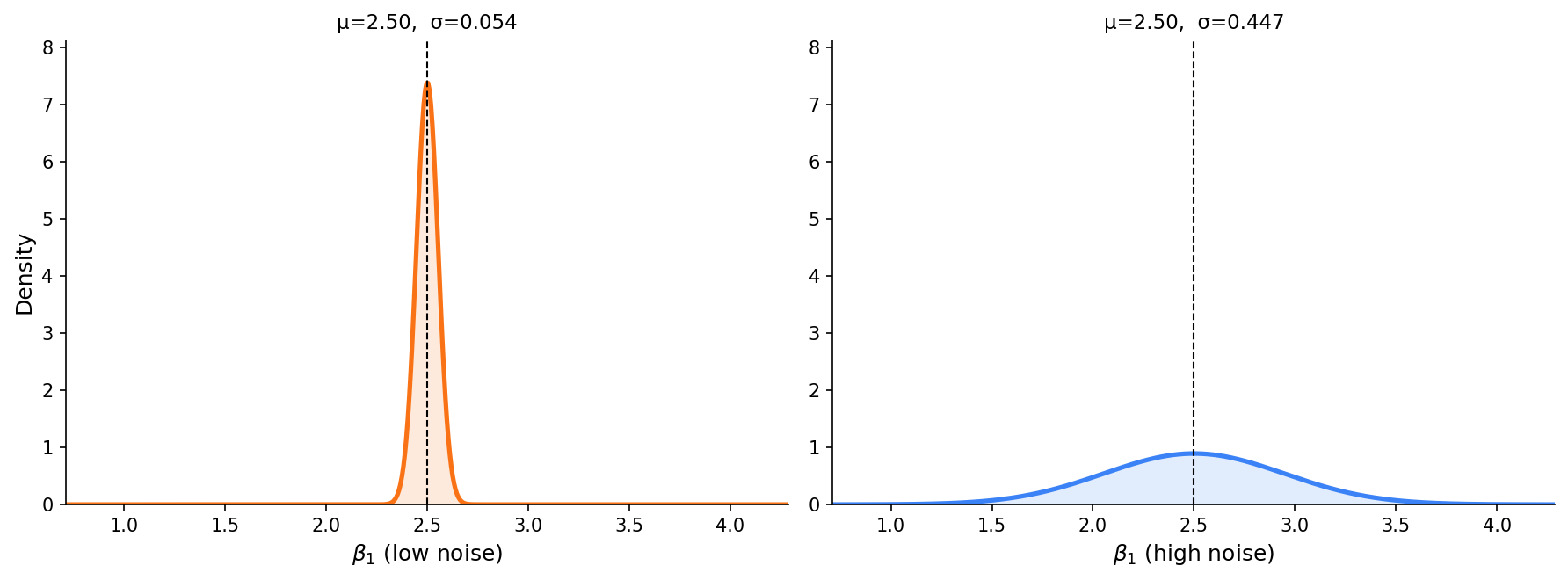
As we observe data points, we apply Bayes’ theorem to update this distribution. Each new point narrows or shifts the posterior. The more data we provide, the more precise our estimate becomes.

This answers the question that frequentist statistics cannot: how probable is it that $\beta_1 = 2.5$? With the low-noise data, very probable. With the high-noise data, it’s the most likely value, but a wide range of slopes are plausible. That distinction matters when making decisions based on the model.

Why It Matters in Practice

The Bayesian approach becomes especially valuable when data is scarce. A frequentist model trained on few observations will produce confident-looking point estimates that are actually quite fragile. Anyone acting on those estimates needs to know how much to trust them.

Another benefit is the prior: a formal mechanism to inject domain knowledge you already have before seeing data. If you know from experience that a slope is unlikely to be negative, you encode that in the prior. The posterior will reflect both your belief and the data, weighting each by how much information they carry.

The tradeoff is computational cost. Computing the posterior is done with approximation methods like Markov Chain Monte Carlo (MCMC) or Variational Inference. That’s a topic for a separate post.

Where to Get Started

To start practicing bayesian learning for small datasets, try Probabilistic Programming. I recommend the PyMC library.